ML QuestionPaper Solution Dec 2023 – AI-DS/ML

Q.1 Solve any Four

A. Explain SVD and its applications. [05] ML

Singular Value Decomposition (SVD) is a powerful matrix factorization technique with various applications across different domains. Here are some common applications of SVD:

Dimensionality Reduction:

SVD can be used for dimensionality reduction in datasets with high-dimensional features. By retaining only the top-k singular values and their corresponding singular vectors, SVD can approximate the original data matrix with reduced dimensions. This is particularly useful for tasks such as image compression, text mining, and recommender systems.

Image Compression:

In image processing, SVD can be applied to compress images while preserving important information. By decomposing the image matrix into its singular values and vectors, low-rank approximations can be generated, leading to significant compression without losing visual quality.

Recommender Systems:

SVD is widely used in collaborative filtering-based recommender systems to make personalized recommendations. By decomposing the user-item interaction matrix into latent factors (represented by singular vectors), SVD can capture underlying patterns in the data and predict users’ preferences for items they have not yet interacted with.

Data Denoising:

SVD can be used for denoising noisy data by filtering out the noise components. By retaining only the dominant singular values and their corresponding singular vectors, SVD can separate the signal from the noise, leading to cleaner data representations.

Latent Semantic Analysis (LSA):

In natural language processing (NLP), SVD is applied in Latent Semantic Analysis (LSA) to uncover hidden semantic structures in text documents. By decomposing the term-document matrix into latent topics, SVD enables document clustering, information retrieval, and text summarization.

Face Recognition:

SVD is used in facial recognition systems to extract important features from face images. By decomposing the face image matrix into its singular values and vectors, SVD can identify unique facial features and reduce the dimensionality of the face space, making it easier to compare and recognize faces.

Principal Component Analysis (PCA):

PCA is a dimensionality reduction technique closely related to SVD. PCA utilizes the eigenvectors of the covariance matrix of the data, which can be obtained through SVD. PCA is widely used for feature extraction, data visualization, and noise reduction in various applications.

Signal Processing:

SVD plays a crucial role in signal processing tasks such as noise reduction, channel equalization, and system identification. By decomposing the signal matrix into its singular values and vectors, SVD can reveal important signal characteristics and aid in signal reconstruction and analysis.

B. Differentiate between supervised and unsupervised learning. [05]

	Supervised Learning	Unsupervised Learning
Input Data	Uses Known and Labeled Data as input	Uses Unknown Data as input
Computational Complexity	Less Computational Complexity	More Computational Complex
Real-Time	Uses off-line analysis	Uses Real-Time Analysis of Data
Number of Classes	The number of Classes is known	The number of Classes is not known
Accuracy of Results	Accurate and Reliable Results	Moderate Accurate and Reliable Results
Output data	The desired output is given.	The desired, output is not given.
Model	In supervised learning it is not possible to learn larger and more complex models than in unsupervised learning	In unsupervised learning it is possible to learn larger and more complex models than in supervised learning
Training data	In supervised learning training data is used to infer model	In unsupervised learning training data is not used.
Another name	Supervised learning is also called classification.	Unsupervised learning is also called clustering.
Test of model	We can test our model.	We can not test our model.
Example	Optical Character Recognition	Find a face in an image.

C. Explain Hebbian Learning rule. [05]

Hebbian Learning Rule, also known as Hebb Learning Rule, was proposed by Donald O Hebb. It is one of the first and also easiest learning rules in the neural network. It is used for pattern classification. It is a single layer neural network, i.e. it has one input layer and one output layer. The input layer can have many units, say n. The output layer only has one unit. Hebbian rule works by updating the weights between neurons in the neural network for each training sample.

Hebbian Learning Rule Algorithm :

Set all weights to zero, w_i= 0 for i=1 to n, and bias to zero.
For each input vector, S(input vector) : t(target output pair), repeat steps 3-5.
Set activations for input units with the input vector X_i = S_i for i = 1 to n.
Set the corresponding output value to the output neuron, i.e. y = t.
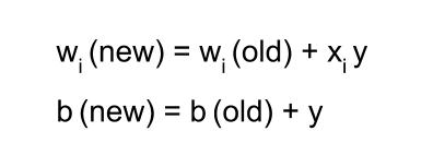
Update weight and bias by applying Hebb rule for all i = 1 to n:

D. Explain the Perceptron model with Bias. [05]

Answer : https://www.doubtly.in/q/explain-perceptron-model-bias/

E. Differentiate between Ridge and Lasso Regression. [05]

Ridge Regression	Lasso Regression
Shrinks the coefficients toward zero	Encourages some coefficients to be exactly zero
Adds a penalty term proportional to the sum of squared coefficients	Adds a penalty term proportional to the sum of absolute values of coefficients
Does not eliminate any features	Can eliminate some features
Suitable when all features are importantly	Suitable when some features are irrelevant or redundant
More computationally efficient	Less computationally efficient
Requires setting a hyperparameter	Requires setting a hyperparameter
Performs better when there are many small to medium-sized coefficients	Performs better when there are a few large coefficients

Q.2 Solve the following

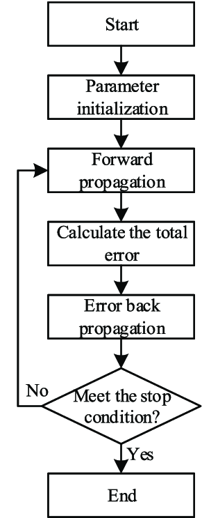
A. Draw a block diagram of the Error Back Propagation Algorithm and explain with a flowchart the Error Back Propagration concept . [10]

The Error Back Propagation Algorithm, commonly referred to as Backpropagation, is a fundamental algorithm used for training artificial neural networks. It is a supervised learning algorithm that aims to minimize the error between the predicted outputs and the actual outputs by adjusting the weights of the network.

Neural Network Structure:
- Input Layer: Receives input features.
- Hidden Layers: Intermediate layers where computations are performed.
- Output Layer: Produces the final output.
Weights and Biases: Parameters that the algorithm adjusts to minimize the error.
Activation Function: A non-linear function (like Sigmoid, ReLU, Tanh) applied to the neuron’s output to introduce non-linearity into the model.
Loss Function: Measures the difference between the predicted output and the actual output (e.g., Mean Squared Error, Cross-Entropy Loss).

Steps in Backpropagation

Initialization: Randomly initialize weights and biases.
Forward Propagation:
- Compute the output of each neuron from the input layer to the output layer.
- For each layer, apply the activation function to the weighted sum of inputs.
Compute Loss: Calculate the error using the loss function.
Backward Propagation:
- Compute the gradient of the loss function with respect to each weight by applying the chain rule of calculus.
- This involves:
- Output Layer: Calculate the gradient of the loss with respect to the output.
- Hidden Layers: Backpropagate the gradient to previous layers, updating the weights and biases.
Update Weights:
- Adjust weights and biases using gradient descent or an optimization algorithm (like Adam, RMSprop).
- Update rule:
  [
  w = w – \eta \frac{\partial L}{\partial w}
  ]
  where ( \eta ) is the learning rate, ( w ) is the weight, and ( \frac{\partial L}{\partial w} ) is the gradient of the loss with respect to the weight.
Iterate: Repeat the forward and backward pass for a number of epochs or until convergence.

Practical Considerations

Learning Rate: A critical hyperparameter that needs to be set properly. Too high can lead to divergence, too low can slow convergence.
Overfitting: Use techniques like regularization (L1, L2), dropout, or early stopping to prevent overfitting.
Gradient Vanishing/Exploding: Deep networks may suffer from these issues. Techniques like Batch Normalization, appropriate activation functions (ReLU), and gradient clipping help mitigate them.

B. Find a linear regression equation for the following two sets of data:

X	Y
3	12
5	18
7	24
9	30

Answer : https://www.doubtly.in/q/find-linear-regression-equation-sets-data-10/

Q.3 Solve the following

A. Diagonalize the matrix A

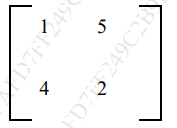
Answer : https://www.doubtly.in/q/diagonalize-matrix-1-5-4-2/

B. Write a short note on overfitting and underfitting of a model. [05]

Underfitting in Machine Learning

Underfitting occurs when a statistical model or machine learning algorithm is too simple to capture the complexities of the data. This results in poor performance on both the training and testing data. An underfit model fails to learn the underlying patterns in the training data, leading to inaccurate predictions, especially on new, unseen examples. Underfitting is typically associated with high bias and low variance, often caused by overly simplified models with basic assumptions.

Reasons for Underfitting:

Overly Simple Model: The model lacks the capacity to represent the data’s complexities.
Inadequate Feature Representation: The input features do not sufficiently capture the factors influencing the target variable.
Insufficient Training Data: The dataset is too small to allow the model to learn effectively.
Excessive Regularization: Over-regularizing to avoid overfitting can overly constrain the model.
Unscaled Features: Features not appropriately scaled can hinder the model’s ability to learn.

Techniques to Reduce Underfitting:

Increase Model Complexity: Use models with more parameters or layers.
Enhance Feature Engineering: Add more relevant features to better capture underlying patterns.
Remove Noise: Clean the data to reduce irrelevant information.
Increase Training Duration: Train the model for more epochs to allow better learning.

Overfitting in Machine Learning

Overfitting occurs when a model performs exceptionally well on the training data but fails to generalize to new, unseen data. This happens when the model learns not only the underlying patterns but also the noise and outliers in the training data, resulting in high variance and poor performance on test data. Overfitting is often seen with complex models that have too much flexibility.

Reasons for Overfitting:

High Variance, Low Bias: The model captures too much detail from the training data.
Excessive Model Complexity: The model has too many parameters relative to the amount of training data.
Insufficient Training Data: The model learns noise due to a lack of diverse training examples.

Techniques to Reduce Overfitting:

Improve Training Data Quality: Ensure the data is clean and representative of the problem.
Increase Training Data Size: More data helps the model generalize better.
Reduce Model Complexity: Simplify the model by reducing the number of parameters or layers.
Early Stopping: Stop training once the performance on validation data starts to degrade.
Regularization Techniques: Use Ridge (L2) or Lasso (L1) regularization to penalize large coefficients.
Dropout in Neural Networks: Randomly drop units during training to prevent co-adaptation.

C. What are activation functions? Explain Binary, Bipolar, Continuous, and Ramp activation functions. [10]

Activation functions are mathematical functions applied to the output of each neuron in a neural network. They introduce non-linearity into the network, enabling it to learn complex patterns in the data. Here’s an explanation of the Binary, Bipolar, Continuous, and Ramp activation functions:

Binary Activation Function:

The binary activation function outputs either 0 or 1 based on a threshold. If the input is below the threshold, it outputs 0; if it’s equal to or above the threshold, it outputs 1.
Mathematically:
[ f(x) = \begin{cases} 0 & \text{if } x < \text{threshold} \ 1 & \text{if } x \geq \text{threshold} \end{cases} ]
This function is typically used in binary classification tasks where the output should represent one of two classes.

Bipolar Activation Function:

The bipolar activation function outputs either -1 or 1 based on a threshold. If the input is below the threshold, it outputs -1; if it’s equal to or above the threshold, it outputs 1.
Mathematically:
[ f(x) = \begin{cases} -1 & \text{if } x < \text{threshold} \ 1 & \text{if } x \geq \text{threshold} \end{cases} ]
Similar to the binary activation function, but it allows for representation of negative values.

Continuous Activation Function:

The continuous activation function produces a smooth, continuous output over the entire range of inputs. Examples include sigmoid and hyperbolic tangent (tanh) functions.
Sigmoid function: [ f(x) = \frac{1}{1 + e^{-x}} ]
Tanh function: [ f(x) = \frac{e^x – e^{-x}}{e^x + e^{-x}} ]
These functions are commonly used in hidden layers of neural networks for their smoothness and suitability for gradient-based optimization algorithms like backpropagation.

Ramp Activation Function:

The ramp activation function linearly increases the output as the input increases up to a certain threshold, after which it saturates to a constant value.
Mathematically:
[ f(x) = \begin{cases} x & \text{if } x < \text{threshold} \ \text{constant} & \text{if } x \geq \text{threshold} \end{cases} ]
This function can be useful in situations where the network needs to gradually activate neurons based on input strength, such as in certain types of regression tasks.

These activation functions serve different purposes and are chosen based on the requirements of the neural network architecture and the nature of the problem being solved.

Q.4 Solve the following

A. Explain Least-Squares Regression for classification. [10]

B. What is the curse of dimensionality? Explain the PCA dimensionality reduction technique in detail. [10]

Handling the high-dimensional data is very difficult in practice, commonly known as the curse of dimensionality. If the dimensionality of the input dataset increases, any machine learning algorithm and model becomes more complex. As the number of features increases, the number of samples also gets increased proportionally, and the chance of overfitting also increases. If the machine learning model is trained on high-dimensional data, it becomes overfitted and results in poor performance.

Hence, it is often required to reduce the number of features, which can be done with dimensionality reduction.

Principal Component Analysis is an unsupervised learning algorithm that is used for the dimensionality reduction in machine learning. It is a statistical process that converts the observations of correlated features into a set of linearly uncorrelated features with the help of orthogonal transformation. These new transformed features are called the Principal Components. It is one of the popular tools that is used for exploratory data analysis and predictive modeling. It is a technique to draw strong patterns from the given dataset by reducing the variances.

PCA generally tries to find the lower-dimensional surface to project the high-dimensional data.

PCA works by considering the variance of each attribute because the high attribute shows the good split between the classes, and hence it reduces the dimensionality. Some real-world applications of PCA are image processing, movie recommendation system, optimizing the power allocation in various communication channels. It is a feature extraction technique, so it contains the important variables and drops the least important variable.

The PCA algorithm is based on some mathematical concepts such as:

Variance and Covariance
Eigenvalues and Eigen factors

Steps for PCA algorithm

Getting the dataset
Firstly, we need to take the input dataset and divide it into two subparts X and Y, where X is the training set, and Y is the validation set.
Representing data into a structure
Now we will represent our dataset into a structure. Such as we will represent the two-dimensional matrix of independent variable X. Here each row corresponds to the data items, and the column corresponds to the Features. The number of columns is the dimensions of the dataset.
Standardizing the data
In this step, we will standardize our dataset. Such as in a particular column, the features with high variance are more important compared to the features with lower variance.
If the importance of features is independent of the variance of the feature, then we will divide each data item in a column with the standard deviation of the column. Here we will name the matrix as Z.
Calculating the Covariance of Z
To calculate the covariance of Z, we will take the matrix Z, and will transpose it. After transpose, we will multiply it by Z. The output matrix will be the Covariance matrix of Z.
Calculating the Eigen Values and Eigen Vectors
Now we need to calculate the eigenvalues and eigenvectors for the resultant covariance matrix Z. Eigenvectors or the covariance matrix are the directions of the axes with high information. And the coefficients of these eigenvectors are defined as the eigenvalues.
Sorting the Eigen Vectors
In this step, we will take all the eigenvalues and will sort them in decreasing order, which means from largest to smallest. And simultaneously sort the eigenvectors accordingly in matrix P of eigenvalues. The resultant matrix will be named as P*.
Calculating the new features Or Principal Components
Here we will calculate the new features. To do this, we will multiply the P* matrix to the Z. In the resultant matrix Z*, each observation is the linear combination of original features. Each column of the Z* matrix is independent of each other.
Remove less or unimportant features from the new dataset.
The new feature set has occurred, so we will decide here what to keep and what to remove. It means, we will only keep the relevant or important features in the new dataset, and unimportant features will be removed out.

Applications of Principal Component Analysis

PCA is mainly used as the dimensionality reduction technique in various AI applications such as computer vision, image compression, etc.
It can also be used for finding hidden patterns if data has high dimensions. Some fields where PCA is used are Finance, data mining, Psychology, etc.

Q.5 Solve the following

A. How to calculate Performance Measures by Measuring the Quality of a model. [10]

Answer : https://www.doubtly.in/q/calculate-performance-measures-measuring-quality-model/

B. Explain the Perceptron Neural Network. [10]

Perceptron is one of the simplest Artificial neural network architectures. It was introduced by Frank Rosenblatt in 1957s. It is the simplest type of feedforward neural network, consisting of a single layer of input nodes that are fully connected to a layer of output nodes. It can learn the linearly separable patterns. it uses slightly different types of artificial neurons known as threshold logic units (TLU). it was first introduced by McCulloch and Walter Pitts in the 1940s.

Types of Perceptron

Single-Layer Perceptron: This type of perceptron is limited to learning linearly separable patterns. effective for tasks where the data can be divided into distinct categories through a straight line.
Multilayer Perceptron: Multilayer perceptrons possess enhanced processing capabilities as they consist of two or more layers, adept at handling more complex patterns and relationships within the data.

Basic Components of Perceptron

A perceptron, the basic unit of a neural network, comprises essential components that collaborate in information processing.

Input Features: The perceptron takes multiple input features, each input feature represents a characteristic or attribute of the input data.
Weights: Each input feature is associated with a weight, determining the significance of each input feature in influencing the perceptron’s output. During training, these weights are adjusted to learn the optimal values.
Summation Function: The perceptron calculates the weighted sum of its inputs using the summation function. The summation function combines the inputs with their respective weights to produce a weighted sum.
Activation Function: The weighted sum is then passed through an activation function. Perceptron uses Heaviside step function functions. which take the summed values as input and compare with the threshold and provide the output as 0 or 1.
Output: The final output of the perceptron, is determined by the activation function’s result. For example, in binary classification problems, the output might represent a predicted class (0 or 1).
Bias: A bias term is often included in the perceptron model. The bias allows the model to make adjustments that are independent of the input. It is an additional parameter that is learned during training.
Learning Algorithm (Weight Update Rule): During training, the perceptron learns by adjusting its weights and bias based on a learning algorithm. A common approach is the perceptron learning algorithm, which updates weights based on the difference between the predicted output and the true output.

Q.6

A. Discuss the various steps of developing a Machine Learning Application. [10]

Machine Learning (ML) is a subset of artificial intelligence (AI) that focuses on enabling machines to learn from data without explicit programming. It allows computers to automatically learn and improve from experience, uncover patterns in data, and make predictions or decisions based on that data.

Steps in Developing a Machine Learning Application:

Collect Data: Gather relevant data from various sources.
Prepare Input Data: Clean, preprocess, and format the collected data for analysis.
Analyze Input Data: Explore and understand the data to identify patterns, trends, and relationships.
Train Algorithm: Select and train the machine learning algorithm(s) on the prepared data.
Test Algorithm: Evaluate the performance of the trained algorithm(s) using test data to ensure accuracy and generalization.
Use Algorithm: Deploy the trained algorithm(s) for making predictions or decisions in real-world applications.
Predict and Revise: Utilize the algorithm(s) to generate predictions or outcomes, and revisit the model periodically for updates and improvements based on new data or feedback.

B. Write a short note on LMS-Widrow Hoff. [05]

Answer here : https://www.doubtly.in/q/draw-delta-learning-rule-lms-widrow-hoff-model/

C. Explain the Maximization algorithm for clustering. [05]

The Expectation-Maximization (EM) algorithm is defined as the combination of various unsupervised machine learning algorithms, which is used to determine the local maximum likelihood estimates (MLE) or maximum a posteriori estimates (MAP) for unobservable variables in statistical models. Further, it is a technique to find maximum likelihood estimation when the latent variables are present. It is also referred to as the latent variable model.

A latent variable model consists of both observable and unobservable variables where observable can be predicted while unobserved are inferred from the observed variable. These unobservable variables are known as latent variables.

Key Points:

It is known as the latent variable model to determine MLE and MAP parameters for latent variables.
It is used to predict values of parameters in instances where data is missing or unobservable for learning, and this is done until convergence of the values occurs.

EM Algorithm

The EM algorithm is the combination of various unsupervised ML algorithms, such as the k-means clustering algorithm. Being an iterative approach, it consists of two modes. In the first mode, we estimate the missing or latent variables. Hence it is referred to as the Expectation/estimation step (E-step). Further, the other mode is used to optimize the parameters of the models so that it can explain the data more clearly. The second mode is known as the maximization-step or M-step.

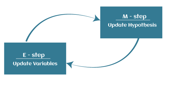
Expectation step (E – step): It involves the estimation (guess) of all missing values in the dataset so that after completing this step, there should not be any missing value.
Maximization step (M – step): This step involves the use of estimated data in the E-step and updating the parameters.
Repeat E-step and M-step until the convergence of the values occurs.

The primary goal of the EM algorithm is to use the available observed data of the dataset to estimate the missing data of the latent variables and then use that data to update the values of the parameters in the M-step.

Table of Contents