IVP Question paper solution may 2023 – AI&DS

IVP Question paper solution may 2023

Q1 a Compare Lossless Compression Techniques & Lossy Compression Techniques [5]

S.NO	Lossy Compression	Lossless Compression
1.	Lossy compression is the method which eliminate the data which is not noticeable.	While Lossless Compression does not eliminate the data which is not noticeable.
2.	In Lossy compression, A file does not restore or rebuilt in its original form.	While in Lossless Compression, A file can be restored in its original form.
3.	In Lossy compression, Data’s quality is compromised.	But Lossless Compression does not compromise the data’s quality.
4.	Lossy compression reduces the size of data.	But Lossless Compression does not reduce the size of data.
5.	Algorithms used in Lossy compression are: Transform coding, Discrete Cosine Transform, Discrete Wavelet Transform, fractal compression etc.	Algorithms used in Lossless compression are: Run Length Encoding, Lempel-Ziv-Welch, Huffman Coding, Arithmetic encoding etc.
6.	Lossy compression is used in Images, audio, video.	Lossless Compression is used in Text, images, sound.
7.	Lossy compression has more data-holding capacity.	Lossless Compression has less data-holding capacity than Lossy compression technique.
8.	Lossy compression is also termed as irreversible compression.	Lossless Compression is also termed as reversible compression.

Q1 b State and Explain properties of FFT. [5]

Answer here : https://www.doubtly.in/q/q1-state-explain-properties-fft-5/

Q1 c Explain zero memory enhancement techniques 1) Contrast Stretching 2) Thresholding [5]  

Zero memory enhancement techniques are methods used in image processing to enhance the visual quality of an image without considering its spatial context. Two common techniques are Contrast Stretching and Thresholding.

1. Contrast Stretching

Contrast stretching, also known as normalization, improves the contrast of an image by expanding the range of pixel intensity values. It maps the original intensity values to a new range, typically from the minimum to maximum possible values, making the details in the image more distinguishable. This is achieved through a linear transformation:

[ I_{\text{new}} = \frac{(I_{\text{old}} – I_{\text{min}})}{(I_{\text{max}} – I_{\text{min}})} \times (L_{\text{max}} – L_{\text{min}}) + L_{\text{min}} ]

where ( I_{\text{old}} ) is the original intensity, ( I_{\text{new}} ) is the adjusted intensity, ( I_{\text{min}} ) and ( I_{\text{max}} ) are the minimum and maximum intensities in the original image, and ( L_{\text{min}} ) and ( L_{\text{max}} ) are the minimum and maximum intensity limits for the desired output.

2. Thresholding

Thresholding is a technique used to convert a grayscale image into a binary image. It involves selecting a threshold value ( T ), and then transforming each pixel in the image as follows:

[ I_{\text{binary}}(x, y) =
\begin{cases}
0 & \text{if } I(x, y) < T \
1 & \text{if } I(x, y) \geq T
\end{cases}
]

where ( I(x, y) ) is the intensity of the pixel at coordinates ( (x, y) ). This technique highlights certain features within the image, such as edges or areas of interest, by separating the pixels into two groups based on the threshold, effectively simplifying the image analysis.

etc resources for it : https://www.dynamsoft.com/blog/insights/image-processing/image-processing-101-point-operations/

Q1 d Find the DCT of the given sequence. f(x)= {1,2,4.7} [5]

Answer here : https://www.doubtly.in/q/find-dct-sequence-fx-124-7/

Q1 e Explain sampling and Quantization. [5]

Sampling and Quantization

Sampling and quantization are two fundamental processes involved in converting an analog signal into a digital signal. These processes are essential in various applications, including digital imaging, audio recording, and telecommunications.

1. Sampling

Sampling is the process of converting a continuous-time signal (analog signal) into a discrete-time signal. This involves measuring the amplitude of the analog signal at regular intervals called the sampling interval. The result is a series of discrete values that represent the signal at those specific points in time.

Key Concepts:

• Sampling Rate (Frequency): The number of samples taken per second, measured in Hertz (Hz). According to the Nyquist theorem, the sampling rate must be at least twice the highest frequency present in the signal to accurately capture all the information without aliasing.
• Nyquist Theorem: To avoid aliasing (distortion due to undersampling), the sampling rate 𝑓𝑠fs​ must be at least twice the maximum frequency 𝑓maxfmax​ of the signal: 𝑓𝑠≥2𝑓maxfs​≥2fmax​.

Example:

• If an audio signal has a maximum frequency of 20 kHz, the minimum sampling rate should be 40 kHz to capture the signal without aliasing.

2. Quantization

Quantization is the process of mapping the continuous range of amplitude values of the sampled signal into a finite set of discrete levels. Each sampled value is approximated to the nearest quantization level, introducing a quantization error.

Key Concepts:

• Quantization Levels: The number of discrete amplitude levels available. More levels result in higher precision but require more bits to represent each sample.
• Bit Depth: The number of bits used to represent each quantized value. Higher bit depth provides a more accurate representation of the analog signal. For example, an 8-bit system has 256 (2^8) levels, while a 16-bit system has 65,536 (2^16) levels.
• Quantization Error: The difference between the actual analog value and the quantized value. This error introduces noise into the signal, known as quantization noise.

Example:

• In an 8-bit quantization system, the continuous amplitude range of the signal (e.g., 0 to 5 volts) is divided into 256 discrete levels. Each sampled value is then approximated to the nearest of these 256 levels.

2 a Explain split and merge segmentation Technique. [10]

Split and merge segmentation is a method used in image processing for dividing an image into regions based on certain criteria, followed by merging those regions to form larger, more meaningful segments.

Splitting Phase:

1. Initial Partitioning: The image is initially divided into smaller regions, typically using a recursive approach such as quadtree decomposition. Each region represents a segment.
2. Region Homogeneity Test: Each small region’s homogeneity is tested based on criteria like color similarity, intensity, texture, or other features. If a region is considered homogeneous (i.e., its pixels are similar enough), it is not split further.

Merging Phase:

1. Adjacent Region Comparison: Adjacent regions are compared to determine if they are similar enough to be merged.
2. Merge Criterion: A merge criterion is applied to determine whether the adjacent regions meet the similarity requirements for merging. This criterion could involve comparing average color values, texture features, or other properties.
3. Merging Process: If adjacent regions pass the merge criterion, they are merged into larger segments. This process continues iteratively until no further merging is possible.

Advantages:

• Reduced Complexity: Splitting into smaller regions reduces the complexity of the segmentation problem.
• Homogeneous Segments: Produces segments with high internal homogeneity.
• Adaptive to Image Content: Can adapt to various types of images and textures.

Limitations:

• Computational Complexity: Recursive splitting and merging can be computationally intensive, especially for large images.
• Over-Segmentation: In some cases, regions may be split excessively, leading to over-segmentation.
• Sensitivity to Parameters: Performance can depend heavily on the choice of parameters and the homogeneity criteria used.

Application:

• Medical Imaging: Identifying different tissues or organs in medical images.
• Satellite Imagery: Segmenting land cover types or identifying objects of interest.
• Object Detection: Preprocessing step for detecting and recognizing objects in computer vision applications.

You can add an numerical as an example too

Split and merge segmentation involves dividing an image into smaller regions based on homogeneity/predicate test during the split phase, and then merging adjacent regions that meet similarity criteria during the merge phase, striking a balance between complexity reduction and content adaptability in image analysis.

2 b What do you mean by redundancy in digital image? Explain image compression model. [10] 

Redundancy in digital image

Redundancy refers to “storing extra information to represent a quantity of information”. So that is the redundancy of data now apply this concept on digital images we know that computer store the images in pixel values so sometimes image has duplicate pixel values or maybe if we remove some of the pixel values they don’t affect the information of an actual image. Data Redundancy is one of the fundamental component of Data Compression.

In digital images, redundancy arises due to various factors, primarily related to the correlation between neighboring pixels and different color channels. Here are the three main types of redundancy:

1. Spatial Redundancy:
   • Spatial redundancy occurs due to correlations between neighboring pixel values within the same image.
   • In most images, adjacent pixels tend to have similar color values, leading to redundant information.
   • Techniques such as spatial domain filtering, which smooths or averages neighboring pixel values, can effectively reduce spatial redundancy.
2. Spectral Redundancy:
   • Spectral redundancy refers to correlations between different color planes or spectral bands within the same image.
   • For example, in color images, there is often redundancy among the color components (e.g., red, green, blue) since they may contain similar information.
   • Transform-based methods like the Discrete Cosine Transform (DCT) or Discrete Wavelet Transform (DWT) are commonly used to decorrelate spectral components and minimize redundancy.
3. Temporal Redundancy:
   • Temporal redundancy applies specifically to video sequences and refers to correlations between successive frames.
   • Since consecutive frames in a video sequence often share similar content, there is redundancy between adjacent frames.
   • Predictive coding techniques, such as motion estimation and compensation, exploit temporal redundancy by predicting the content of subsequent frames based on previous ones.

Image compression models

Image compression models are algorithms or systems designed to reduce the size of digital images while preserving their visual quality to some extent. These models can be broadly categorized into two types: lossy compression and lossless compression.

1. Lossy Compression: In lossy compression, some data from the original image is discarded during the compression process to achieve higher compression ratios. This means that when the image is decompressed, it won’t be identical to the original. However, the goal is to remove data that is less perceptible to the human eye, minimizing the loss in visual quality. Lossy compression is commonly used in scenarios where storage space or bandwidth is limited, such as on the internet or in multimedia applications.
2. Lossless Compression: Unlike lossy compression, lossless compression algorithms reduce the size of an image without losing any information from the original. This means that when the image is decompressed, it is identical to the original. Lossless compression is often preferred in scenarios where preserving every detail of the image is critical, such as in medical imaging or graphic design.

A typical image compression model consists of two main components:

• Encoder/Compressor: This component takes the original image as input and applies various compression techniques to reduce its size. In lossy compression, this may involve techniques like quantization (reducing the number of colors or levels of detail), transform coding (using mathematical transforms like Discrete Cosine Transform), or predictive coding (predicting pixel values based on neighboring pixels). In lossless compression, techniques like run-length encoding, Huffman coding, or Lempel-Ziv-Welch (LZW) compression may be used. The compressed data produced by the encoder is often significantly smaller in size compared to the original image.
• Decoder/Decompressor: This component takes the compressed data generated by the encoder and reverses the compression process to reconstruct the original image. In lossy compression, the reconstructed image will not be identical to the original due to the loss of some data during compression. However, the goal is to ensure that the visual quality of the reconstructed image is acceptable to human observers. In lossless compression, the reconstructed image is bit-for-bit identical to the original.

These encoder and decoder components work together to achieve efficient compression and decompression of digital images while balancing between compression ratio and visual quality, depending on whether lossy or lossless compression is used.

3 a Find DFT of the given image using DIT-FFT.

0 1 2 1 
1 2 3 2 
3 3 4 3 
1 2 3 2 

Answer : https://www.doubtly.in/q/3-find-dft-image-dit-fft/

3 b Equalize the given histogram[10]  

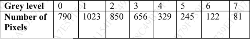
Solution : https://www.doubtly.in/q/equalize-histogram/

4a Write short note on fast hadamard transform [10]

Answer : https://www.doubtly.in/q/write-short-note-fast-hadamard-transform/

4 b Explain in detail low pass (smoothing) filters. [10]

Low pass filters, also known as smoothing filters, are signal processing tools used to remove high-frequency noise from a signal while retaining the low-frequency components. They allow the passage of signals with frequencies below a certain cutoff frequency while attenuating signals with frequencies above this cutoff.

Low pass (smoothing) filters:

1. Basic Principle: The basic principle behind a low pass filter is to average out or attenuate the high-frequency components of a signal while preserving the low-frequency components. This is achieved by employing a filter kernel or function that emphasizes low-frequency components and suppresses high-frequency ones.
2. Frequency Response: Low pass filters have a frequency response that exhibits high attenuation for frequencies above a certain cutoff frequency and relatively low attenuation for frequencies below this cutoff. The cutoff frequency is a critical parameter that determines the point at which the filter begins to attenuate the signal.
3. Types of Low Pass Filters:

• Ideal Low Pass Filter: This theoretical filter provides perfect attenuation above the cutoff frequency and perfect preservation of frequencies below the cutoff. However, it’s impossible to implement in practice due to its idealized nature.
• Butterworth Filter: Butterworth filters are commonly used in practical applications due to their maximally flat frequency response in the passband and smooth transition to the stopband. They are designed to achieve a specified level of attenuation at the cutoff frequency.
• Chebyshev Filter: Chebyshev filters offer steeper roll-off rates than Butterworth filters but introduce ripples in either the passband or the stopband to achieve this. They are useful when a sharper transition between the passband and stopband is required.
• Bessel Filter: Bessel filters provide a nearly linear phase response, making them suitable for applications where phase distortion must be minimized. They offer a slower roll-off compared to Butterworth and Chebyshev filters.

1. Filter Design: The design of a low pass filter involves selecting the appropriate type of filter based on the requirements of the application, such as the desired attenuation at the cutoff frequency, the steepness of the roll-off, and the tolerance for passband and stopband ripples. Design parameters include the filter order (determining the complexity of the filter), the cutoff frequency, and the transition bandwidth.
2. Implementation: Low pass filters can be implemented using various techniques, including analog circuits (such as RC filters), digital signal processing algorithms (such as finite impulse response (FIR) and infinite impulse response (IIR) filters), and software-based methods. Digital filters are particularly common due to their flexibility, ease of implementation, and ability to achieve precise specifications.
3. Applications:

• Signal Smoothing: Removing noise from signals in applications such as audio processing, biomedical signal analysis, and sensor data processing.
• Image Processing: Smoothing images to reduce noise and enhance features in applications like computer vision and medical imaging.
• Communications: Pre-processing signals in communication systems to improve the quality of transmitted data and reduce interference.

5 a Explain edge detection in detail. [10]

Edge detection is a fundamental concept in image processing, aiming to identify and locate abrupt changes in brightness, which often correspond to object boundaries or significant transitions in an image. It plays a pivotal role in various tasks such as pattern recognition, image segmentation, and scene analysis.

Importance of Edge Detection:

1. Localization of Object Boundaries: Edges typically mark the boundaries between different objects or regions within an image. Detecting these edges helps in segmenting objects from the background.
2. Feature Extraction: Edges are essential features of an image, providing crucial information about the shapes and structures present within it. Extracting edges facilitates tasks like object recognition and classification.
3. Image Enhancement: Edge detection can enhance the visual appearance of an image by emphasizing its structural details, making it easier for subsequent analysis and interpretation.

Basic Principle:

The fundamental idea behind edge detection involves applying specific mathematical operators or filters to an image to highlight areas of rapid intensity changes. These changes often manifest as peaks or troughs in the gradient of the image. The process typically includes the following steps:

1. Edge Enhancement: Using operators designed to accentuate local edges, thereby making them more prominent against the background.
2. Edge Strength Estimation: Determining the strength of detected edges based on the magnitude of gradient variations at different points in the image.
3. Edge Point Identification: Setting a threshold to classify points with significant gradient changes as edge points.

Edge Detection Operators:

Several operators are commonly employed for edge detection.

1. Sobel Edge Detection Operator: This operator calculates gradients in both the horizontal (Gx) and vertical (Gy) directions using convolution kernels. The resulting gradient magnitude highlights edges in the image.
2. Robert’s Cross Operator: Similar to the Sobel operator, Robert’s Cross calculates gradients using simple 2×2 convolution kernels. It’s quick to compute and effective for basic edge detection tasks.
3. Laplacian of Gaussian (LoG): This operator combines Gaussian smoothing with the Laplacian operator to detect edges. It first applies Gaussian smoothing to reduce noise sensitivity, followed by Laplacian filtering to highlight regions of rapid intensity changes.
4. Prewitt Operator: Like Sobel, the Prewitt operator computes gradients in both horizontal and vertical directions. It’s computationally efficient and widely used for edge detection.

Limitations and Considerations:

1. Noise Sensitivity: Edge detection is susceptible to noise, which can lead to false detections or inaccuracies. Pre-processing steps like noise reduction are often necessary.
2. Threshold Selection: Setting an appropriate threshold for edge detection is crucial. It affects the sensitivity and specificity of edge detection algorithms.
3. Scale Considerations: Different edge detection methods may perform differently based on the scale of features present in the image. Smoothing or scaling techniques may be necessary for optimal results.

5b Explain Huffman Coding with example. [10]

Detailed answer : https://www.javatpoint.com/huffman-coding-algorithm

6 a Explain Digital video format and estimation in detail.

Digital Video Format:

Digital video format refers to the method by which video data is encoded, stored, and transmitted in a digital format. Unlike analog video, which represents video signals as continuously varying voltages, digital video represents video as discrete digital signals, typically binary data.

1. Encoding: Digital video is encoded using various compression algorithms to reduce file size while maintaining acceptable visual quality. Common digital video formats include MPEG-2, MPEG-4 (including formats like H.264 and H.265), AVI, QuickTime, and WMV (Windows Media Video).
2. Container Format: Digital video files are often packaged within a container format, which encapsulates the video data along with audio, subtitles, and metadata. Examples of container formats include MP4, MOV, AVI, and MKV.
3. Resolution and Frame Rate: Digital video can have different resolutions (such as 720p, 1080p, or 4K) and frame rates (measured in frames per second, fps). Higher resolutions and frame rates generally result in better image quality but also require more storage space and processing power.
4. Compression: Compression is essential for reducing the size of digital video files without significantly degrading visual quality. Compression algorithms remove redundant or unnecessary information from the video stream while preserving important details. There are two types of compression: lossless (which preserves all original data) and lossy (which sacrifices some data to achieve greater compression).
5. Codecs: Codecs (encoder-decoder) are used to encode and decode digital video data. They implement specific compression algorithms and determine how video data is compressed and decompressed. Popular codecs include H.264 (AVC), H.265 (HEVC), MPEG-2, and VP9.
6. Playback Devices: Digital video can be played back on various devices, including computers, smartphones, tablets, media players, and smart TVs. The compatibility of video formats and codecs varies between devices, so it’s essential to choose formats that are widely supported.

Estimation in Digital Video:

Estimation in digital video refers to predicting the amount of storage space required for storing a given video file or stream, as well as estimating the bandwidth needed for transmitting video over a network. This estimation involves several factors:

1. Video Resolution: Higher resolutions require more storage space and bandwidth. Common resolutions include Standard Definition (SD), High Definition (HD), Full HD (1080p), and Ultra HD (4K).
2. Frame Rate: Higher frame rates increase the amount of data per second, requiring more storage space and bandwidth. Common frame rates include 24 fps (cinematic), 30 fps (standard for TV), and 60 fps (high motion).
3. Compression: The choice of codec and compression settings significantly affects the file size and bandwidth requirements. Different codecs offer varying levels of compression efficiency and quality.
4. Duration: The length of the video (in seconds, minutes, or hours) directly impacts the total file size and transmission time.
5. Audio: If the video includes audio, the audio codec, bitrate, and number of channels also contribute to the overall data size.
6. Bitrate: Bitrate refers to the amount of data processed per unit of time and is typically measured in bits per second (bps) or kilobits per second (kbps). Higher bitrates result in better quality but require more storage space and bandwidth.

Estimating the storage and bandwidth requirements for digital video involves considering these factors and selecting appropriate encoding settings to achieve the desired balance between quality, file size, and transmission efficiency. Various online calculators and software tools are available to assist in estimating video file sizes based on input parameters such as resolution, frame rate, codec, and duration.

6b Write short note on  

1) Composite and Component Video 

Composite Video and Component Video are two different methods of transmitting video signals, each with its own characteristics and applications:

1. Composite Video:

• Definition: Composite video combines all video information into a single signal.
• Signal Structure: In composite video, luminance (brightness) and chrominance (color) information are combined into one signal. This means that the entire picture is transmitted as one signal through a single cable.
• Connection: Typically, composite video uses a single RCA connector (yellow) for transmission.
• Quality: Composite video is capable of transmitting standard definition video, but it suffers from signal degradation due to the mixing of luminance and chrominance information. This can result in issues such as color bleeding and reduced image sharpness.
• Common Uses: Composite video was widely used in older consumer electronics devices such as VCRs, early DVD players, and older game consoles.

1. Component Video:

• Definition: Component video separates the video signal into multiple components.
• Signal Structure: Component video splits the video signal into three separate channels: luminance (Y), and two chrominance channels (Cb and Cr). This separation allows for better image quality and color accuracy compared to composite video.
• Connection: Component video typically uses three RCA connectors (red, green, blue) or a set of three cables bundled together.
• Quality: Component video offers higher quality than composite video, capable of transmitting both standard definition and high definition video signals. The separation of luminance and chrominance components reduces signal interference and improves image clarity.
• Common Uses: Component video was commonly used in older high-definition displays, analog television sets, and certain video equipment. It has been largely replaced by digital interfaces like HDMI in newer devices.

Comparison Table:

Aspect	Composite Video	Component Video
Signal Structure	Combines luminance and chrominance	Separates luminance and chrominance
Number of Cables	Single cable (typically RCA)	Three cables (RCA or bundled)
Image Quality	Lower quality, prone to interference	Higher quality, better color accuracy
Resolution Support	Standard definition	Standard and high definition
Connection	Simple, single cable connection	Requires multiple cables
Common Uses	Older consumer electronics	Older high-definition displays

2) BMP Image File Format 

The BMP (Bitmap) image file format is one of the oldest and simplest formats for storing digital images. Originally developed by Microsoft, it is widely supported across different platforms and applications.

1. Basic Structure: BMP files are typically uncompressed raster images, meaning they store data for each individual pixel in the image. Each pixel’s color and position information is stored directly in the file.
2. Header Information: The BMP file begins with a header section that contains essential information about the image, such as its dimensions, color depth, and compression method (if any). This header provides the necessary metadata for properly interpreting the image data.
3. Pixel Data: Following the header, BMP files contain the actual pixel data arranged in rows from top to bottom. Each pixel is represented by a series of bits, with the number of bits per pixel determining the color depth and range of colors available in the image. Common color depths include 1-bit (black and white), 8-bit (256 colors), 24-bit (true color), and 32-bit (true color with alpha channel for transparency).
4. Color Palette: In indexed color BMPs (with color depths less than 24 bits), a color palette is included after the header. This palette contains a list of color values used in the image, with each pixel in the pixel data referring to an index in this palette to determine its color.
5. Compression: While BMP files typically use uncompressed pixel data, there are variations of the format that support compression, such as RLE (Run-Length Encoding). This can reduce file size, but it’s less common compared to compressed formats like JPEG or PNG.
6. Platform Independence: BMP files are platform-independent and can be read and written by most operating systems and image editing software. However, their lack of compression means they tend to have larger file sizes compared to formats like JPEG or PNG, making them less suitable for web usage.
7. Usage: Despite their larger file sizes, BMP files are still used in certain applications where image quality and fidelity are paramount, such as professional graphics editing, medical imaging, and certain types of digital art.

IVP Question paper solution may 2023 – AI&DS