DMBI MU QPaper Solution (Dec 2023)
This solution is contributed by Darshan and Mangesh. Make sure to follow them on their social handles:
- Mangesh Pangam:
- LinkedIn: Mangesh Pangam
- Instagram: @Mangesh_2704
You can also read it here if you want
Q.1 A) Explain types of attributes used in data exploration. (10 marks) Ans-
What is an Attribute?
● The attribute can be defined as a field for storing the data that represents the● characteristics of a data object.
● The attribute is the property of the object.
● The attribute represents different features of the object.
● For example, hair color is the attribute of a lady. Similarly, rollno, and marks are attributes of a student.
● An attribute vector is commonly known as a set of attributes that are usedtodescribe a given object.
Type of attributes:-
1. Qualitative Attributes
⮚ It includes the attributes such as Nominal, Ordinal and Binary 2. Quantitative Attributes
⮚ It includes the attributes such as Discrete and Continuous 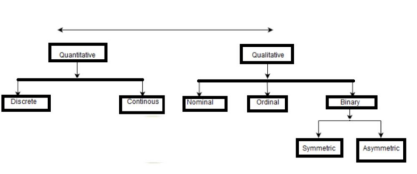
It only provides only attributes sufficient to tell the difference between objects. Suchas name, roll no, address are all different objects used in the dataset. Examples – Eye color (blue, brown, green), Car Brands (Toyota, Honda, Ford, BMW)
2. Ordinal Attribute
It is an attribute whose possible values provide sufficient information to have a meaningful order of objects. Such as salary_range,education_level, ranking etc.
Prepared by Mangesh Pangam(XIE)
Examples – Gender of individuals (e.g., male, female, non-binary), Marital status (e.g., single, married, divorced).
3. Binary Attribute
Binary Attributes are 0 and 1.0 represents the lack of any feature and 1 represents theaddition of specific characteristics.
Examples – Subscription status (e.g., subscribed, not subscribed), Response to a yes/no question (e.g., yes, no).
4. Numeric attribute
It is quantitative in nature i.e.the quantity can be measured and represented in formof integers or real values.
Examples – Age of individuals in a dataset (e.g., 25, 30, 42), Temperature recordedinCelsius (e.g., 22.5°C, 15.3°C).
5. Temporal Attributes
Temporal attributes represent time-related data, such as dates, timestamps, or durations.
Examples – date of birth, time of purchase, and duration of a task.
6. Spatial Attributes
Spatial attributes represent location-based data, such as latitude and longitude coordinates or addresses.
Examples – It is commonly used in geographic information systems (GIS) and location-based services.
7. Derived Attributes
Derived attributes are created from existing attributes through mathematical operations, transformations, or feature engineering techniques.
Examples – Calculating the BMI (Body Mass Index) from height and weight or creating dummy variables from categorical attributes.
Prepared by Mangesh Pangam(XIE)
Q. 1 B) Explain DBSCAN algorithm with example. (10 marks) Ans-
DBSCAN is a clustering algorithm that defines clusters as continuous regions of highdensity and works well if all the clusters are dense enough and well separated by low- density regions. In the case of DBSCAN, instead of guessing the number of clusters, will define two hyperparameters: epsilon and minPoints to arrive at clusters.
1. Epsilon (ε): A distance measure that will be used to locate the points/to checkthe density in the neighbourhood of any point.
2. minPoints(n): The minimum number of points (a threshold) clustered together for a region to be considered dense.
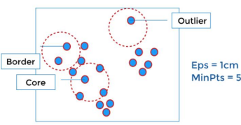
Here’s how DBSCAN works:
1. Core Points: A core point is a data point that has at least minPts points (includingitself) within its ε-neighborhood.
2. Border Points: A border point is not a core point but lies within the ε- neighborhood of a core point.
3. Noise Points: A noise point is neither a core point nor a border point.
The algorithm proceeds as follows:
1. Start with an arbitrary point in the dataset.
2. If the point is a core point, create a new cluster and expand it by adding all reachable points (directly or indirectly) within ε distance to the cluster. 3. Repeat the process for all unvisited core points and their respective clusters. 4. Assign border points to the clusters they border on.
5. Any remaining unvisited points are treated as noise
Prepared by Mangesh Pangam(XIE)
Here’s an example:
Consider a dataset of points plotted on a 2D plane
Dataset:
Point X-coordinate Y-coordinate
1 2 3
2 4 5
3 5 4
4 7 2
5 8 3
6 3 5
7 8 9
8 2 2
9 6 7
10 5 6
Let’s use DBSCAN with ε = 2 and minPts = 3:
⮚ Point 1, 6, and 8 are core points because they have at least 3 points within ε distance.
⮚ Points 2, 3, 4, 5, 9, and 10 are border points as they are within ε distance of a corepoint but do not have enough neighbors to be core points themselves. ⮚ Points 7 is a noise point as it does not meet the criteria of being a core or border point.
The resulting clusters might be:
Cluster 1: {1, 2, 3, 6, 8}
Cluster 2: {4, 5, 9, 10}
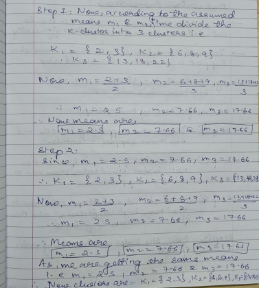
Q.2 A) Explain K means algorithm in detail. Apply K-means Algorithmto dividethe given set of values {2,3,6,8,9,12,15,18,22} into 3 clusters. (10 marks) Ans-
∙ K-means clustering is an algorithm to classify or to group the different object based on attributes or features into K number of group.
∙ K is positive integer number(which can be decided by user) ∙ Define K centroids for K clusters which are generally far away fromeach other.
Prepared by Mangesh Pangam(XIE)
∙ Then group the elements into clusters which are nearer to the centroid of that cluster.
∙ After this first step, again calculate the new centroid for each cluster basedonthe elements of that cluster.
∙ Follow the same method, and group the elements based on new centroid. ∙ In every step, the centroid changes and elements move from one cluster toanother.
∙ Do the same process till no element is moving from one cluster to another.
Given data – {2,3,6,8,9,12,15,18,22}
Let assume:
m1 = 3
m2 = 8
m3 = 18
Prepared by Mangesh Pangam(XIE)
Q.2 B) Compare Bagging and Boosting of a classifier.
Ans-
1. Bagging
Bootstrap Aggregating, also known as bagging, is a machine learning ensemble meta- algorithm designed to improve the stability and accuracy of machine learning algorithms used in statistical classification and regression. It decreases the variance and helps to avoid overfitting. It is usually applied to decision tree methods. Bagging is a special case of the model averaging approach. Description of the Technique
Suppose a set D of d tuples, at each iteration i, a training set Di of d tuples is selectedvia row sampling with a replacement method (i.e., there can be repetitive elements from different d tuples) from D (i.e., bootstrap). Then a classifier model Mi is learnedfor each training set D < i. Each classifier Mi returns its class prediction. The baggedclassifier M* counts the votes and assigns the class with the most votes to X(unknown sample).
Implementation Steps of Bagging
Step 1: Multiple subsets are created from the original data set with equal tuples, selecting observations with replacement.
Step 2: A base model is created on each of these subsets.
Step 3: Each model is learned in parallel with each training set and independent of each other.
Step 4: The final predictions are determined by combining the predictions fromall the models.
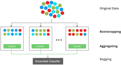
Example of Bagging
The Random Forest model uses Bagging, where decision tree models with higher variance are present. It makes random feature selection to grow trees. Several randomtrees make a Random Forest.
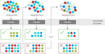
2. Boosting
Boosting is an ensemble modeling technique that attempts to build a strong classifier from the number of weak classifiers. It is done by building a model by using weakmodels in series. Firstly, a model is built from the training data. Then the second model is built which tries to correct the errors present in the first model. This procedure is continued and models are added until either the complete training data set is predicted correctly or the maximum number of models is added. Boosting Algorithm:
1. Initialise the dataset and assign equal weight to each of the data point. 2. Provide this as input to the model and identify the wrongly classified data points. 3. Increase the weight of the wrongly classified data points and decrease the weights
of correctly classified data points. And then normalize the weights of all data points.
4. if (got required results)
Goto step 5
else
Goto step 2
5. End
Differences Between Bagging and Boosting
| Sr.No | Bagging | Boosting |
| 1. | The simplest way of combiningpredictions that belong totype. | A way of combining predictionsthat belong to the different types. the same |
| 2. | Aim to decrease variance, not bias. | Aim to decrease bias, not variance. |
| 3. | Each model receives equal weight. | Models are weighted accordingperformance. |
| 4. | Each model is built independently. | New models are influencedby the performance of previouslymodels. |
| 5. | Different training data subsetsselected using row sampling withreplacement and randommethods from the entire trainingdataset. | Every new subset contains the elements are that were misclassified by previous models. sampling |
| 6. | Bagging tries to solve the over fitting problem. | Boosting tries to reduce bias. |
| 7. | If the classifier is unstablevariance), then apply bagging. | If the classifier is stable and simple (high (high bias) the apply boosting. |
| 8. | In this base classifiers are trainedparallelly. | In this base classifiers are trainedsequentially. |
| 9 | Example: The Randommodel uses Bagging. | Example: The AdaBoost uses Boosting forest techniques |
This solution is contributed by Darshan and Mangesh. Make sure to follow them on their social handles:
- Mangesh Pangam:
- LinkedIn: Mangesh Pangam
- Instagram: @Mangesh_2704
